
Company Default prediction - DLMM Internal Rating Model in R
- Steps followed to implement the DLMM Model in R language
- Step 1 – Converting SPSS formatted data
- Step 2 - One by one empirical analysis of variables
- Step 3 - Cross-tabulation 01STATUS versus Industry Sector Code
- Step 4 - Exploring graphically the probability distribution of a variable
- Step 5 - Testing the normality of the probability distribution of a variable
- Step 6 - Evaluating the good/bad discriminant power of a variable
- Step 7 - Empirical monotonicity of ROE relative to good-bad progression
- Step 8 - Correlation between variable couples
- Step 9 - Analysis of outliers
- Step 10 - Data encoding
- Step 11 - Synoptic table of variable properties
- Step 12 - Linear Discriminant Analysis - Initial approach
- Step 13 - Experimenting with Stepwise Linear Discriminant Analysis
- Step 14 - Gaussian Copula encoding scheme
Step 9 – Analysis of outliers
Purpose
This implementation follows step by step the contents of Chap. 4, section 4.5.8 : Analysis of outliers, pp. 162-164
Method
The authors base their approach on the use of the “interquartile range” (IQR). More precisely they name “outliers”, those samples which values are higher than the 3rd quartile (Q3) and lower than the 1st quartile (Q1).
Computing the number of outliers for the ration ROE (page 163) – -> (https://github.com/MoiraCorp/DLMM-IRating-in-R/tree/main/steps/step9/roeoutlr)
Computing outliers percentage for all the ratios – -> (https://github.com/MoiraCorp/DLMM-IRating-in-R/tree/main/steps/step9/alloutlr)
Masking outlier’s values using the NA R notation – -> (https://github.com/MoiraCorp/DLMM-IRating-in-R/tree/main/steps/step9/naoutlr)
Computing the number of outliers for the ration ROE (page 163)
Following the authors’s approach, we implement the FindOutliers() function in order to to detect extreme outliers
FindOutliers <- function(data) { lowerq = quantile(data, na.rm=TRUE)[2] upperq = quantile(data, na.rm=TRUE)[4] iqr = upperq – lowerq # we identify extreme outliers extreme.threshold.upper = (iqr * 3) + upperq extreme.threshold.lower = lowerq – (iqr * 3) result <- which(data > extreme.threshold.upper | data < extreme.threshold.lower) }
For more information on the detection of outliers in R, see for example: “Outliers detection in R” -> https://statsandr.com/blog/outliers-detection-in-r/
The FindOutliers() function is used to evaluate the percentage of extereme outliers for the ROE variable
The printed output is:extreme.outl <- FindOutliers(wcs2train$ROE) # compute percentage of extreme outliers outlprc = length(extreme.outl)/length(wcs2train$ROE) outlprc
[1] 0.1210692
NOTE : This compares closely with the percentage of 12% indicated by the authors in page 164
We start by sub-setting the ratios from the W_CS_1_AnalysisSampleDataSet_2B.xls table
ratiovars <- c(86:119)
wcs2train.ratios <- wcs2train[ratiovars] sapply(wcs2train.ratios, class)
The percentage of outliers is then computed for all the Ratio variables
for(i in 1:length(wcs2train.ratios)){
# use the function to identify extreme outliers
extreme.outl <- FindOutliers(wcs2train.ratios[,i])
# compute percentage of extreme outliers
outlprc = length(extreme.outl)/length(wcs2train.ratios[,i])
cat(sprintf(“%s, %.2f\n”, colnames(wcs2train.ratios)[i], outlprc))
}
| Ratio | Percentage | Ratio | Percentage | Ratio | Percentage | Ratio | Percentage |
|---|---|---|---|---|---|---|---|
| EXTRIC | 0.24 | SALESONV | 0.13 | ROE | 0.12 | INVENTOR | 0.1 |
NOTE : The results show that: ROE, INVENTOR, EXTRIC and SALESONV do have “outliers” percentage >= 10%
| Ratio | Percentage | Ratio | Percentage | Ratio | Percentage | Ratio | Percentage |
|---|---|---|---|---|---|---|---|
| DEBTEQU | 0.09 | EBITDAIE | 0.09 | RECEIVAB | 0.09 | ROETR | 0.09 |
| DEBTEQUTR | 0.08 | SALESMIN | 0.07 | ROAMINUS | 0.06 | V95A | 0.06 |
| EQUILIABL | 0.05 | EQUITYON | 0.05 | IEONEBIT | 0.05 | IEONFINA. | 0.05 |
| NIEONEBI | 0.05 | ROA | 0.05 | COMMERCI | 0.04 | CURRENT | 0.04 |
| PAYABLES | 0.04 | ROI | 0.04 | ROS | 0.04 | V89A | 0.03 |
| EBITDAON | 0.03 | QUICKRA | 0.02 | TAXESONG | 0.02 | ASSETSTU | 0.01 |
| V94A | 0.01 |
NOTE : It worth pointing out that a few NA (Not available) values are present, principaly in the TAXESONG ratio
| Ratio | Percentage | Ratio | Percentage | Ratio | Percentage | Ratio | Percentage |
|---|---|---|---|---|---|---|---|
| IEONLIAB | 0 | INTANGIB | 0 | TRADERE. | 0 | V110A | 0 |
| TRADEPA. | 0 |
NOTE : The results show anomalies in the computation of the quantiles for IEONLIAB, INTANGIB, TRADERE., V110A and TRADEPA:
- for IEONLIAB it is probably due to the presence of one extreme outlier (value 107.47) for a population ranging 0-23
- for all the other ratios the result is harder to explain
It is common practice to “mask out” outlier values for each of the Ratio variables in order to manipulate more manageable statistical distributions.
It follows the recommendations of the authors in section 4.5.9.1 – Treatment of outliers, page 164.
Here we will mask out the outliers by replacing these values by the NA R notation (Not Available)
wcs2train.ratios.NA <- wcs2train.ratios
for(i in 1:length(wcs2train.ratios.NA)){
# use the function to identify extreme outliers
extreme.outl <- FindOutliers(wcs2train.ratios.NA[,i])
# Replacing extreme outliers values by NA
wcs2train.ratios.NA[,i][extreme.outl] <- NA
cat(sprintf(“%s\n”, colnames(wcs2train.ratios)[i]))
}
In order to graphically evaluate the effects of this ecoding we use the chart.Correlation() from the PerformanceAnalytics R package -> https://cran.r-project.org/web/packages/PerformanceAnalytics/index.html
library(“PerformanceAnalytics”)
chart.Correlation(wcs2train.ratios.NA, histogram=TRUE, pch=19)
The result is illustared in Table_4_21b_Page164_AllvariableswithNA_CoorDiag.pdf
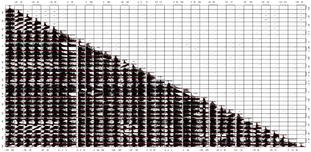
NOTE : In this chart, the cloud points provide far more information than the one presented in the unprocessed datable with outliers present (-> https://github.com/MoiraCorp/DLMM-IRating-in-R/tree/main/steps/step8/alternr)
In order to compute the matrix of p-value, we use the custom cor.pvalue() R function already introduced in chapter “step8”: -> https://github.com/MoiraCorp/DLMM-IRating-in-R/tree/main/steps/step8/selectvar
# Function computing the matrix of p-values
# mat : is a matrix of data
# … : further arguments to pass to the native R cor.test function
cor.pvalue <- function(mat, …) {
mat <- as.matrix(mat)
n <- ncol(mat)
p.mat<- matrix(NA, n, n)
diag(p.mat) <- 0
for (i in 1:(n – 1)) {
for (j in (i + 1):n) {
tmp <- cor.test(mat[, i], mat[, j], …)
p.mat[i, j] <- p.mat[j, i] <- tmp$p.value
}
}
colnames(p.mat) <- rownames(p.mat) <- colnames(mat)
p.mat
}
In order to produce a graphics representation of the Pearson correlation between all NA masqued Ratio Variables we are using the corrplot R package: -> https://cran.r-project.org/web/packages/corrplot/vignettes/corrplot-intro.html
library(corrplot)
corrprs <- cor(wcs2train.ratios.NA, use=”pairwise”, method=”pearson”)
p.mat <- cor.pvalue(wcs2train.ratios.NA)
col <- colorRampPalette(c(“#BB4444”, “#fcc3b8”, “#FFFFFF”, “#add2f7”, “#4fc69d”))
corrplot(corrprs, method=”color”, col=col(200),
type=”upper”,
addCoef.col = “black”, # Add coefficient of correlation
addCoefasPercent = TRUE,
tl.col=”black”, tl.srt=45, #Text label color and rotation
# Combine with significance
p.mat = p.mat, sig.level = 0.01, insig = “blank”,
# hide correlation coefficient on the principal diagonal
diag=FALSE
)
The graphics representation of the Pearson correlation between all Na masqued Ratio Variables is presented in Table_4_21c_Page 164_RatioswithNA_Correlation.pdf
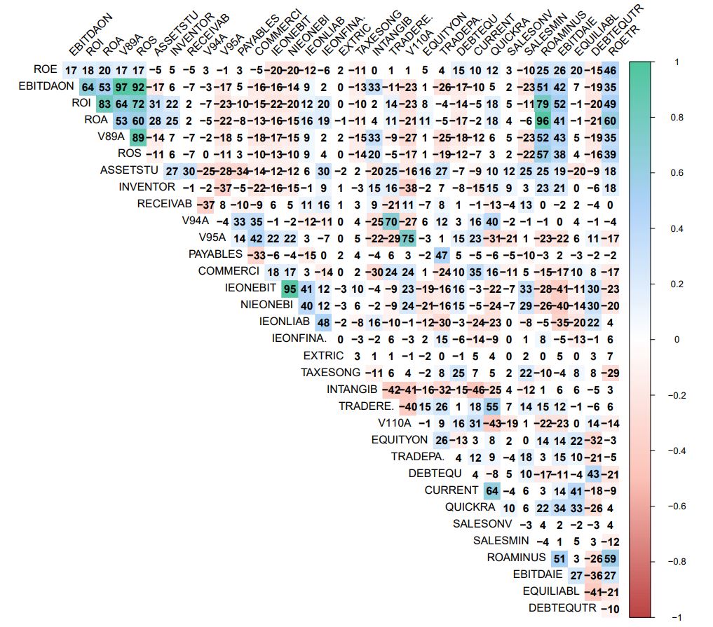
NOTE : When comparing with the same diagram obtained in step 8 -> https://github.com/MoiraCorp/DLMM-IRating-in-R/tree/main/steps/step8/allvar
it appears that, though groups of correlated variables do appear again in the new display, there are some remarquable differences
GR1: this ROE, ROETR, DEBTEQUTR group does not appear any more
GR2: EBITDAON, V89A (97% with EBITDAON), ROS (92% with EBITDAON)
| Column in R table | Code in text | Description |
|---|---|---|
| EBITDAON-87 | EBITDAonSALES | Ratio EBITDA/Sales [%] |
| V89A-90 | EBITDAonVP | Ratio EBITDA/Value of Production |
| ROS-91 | ROS | Ratio EBIT/Sales [%] |
GR3: ROI, ROA (83% with ROI) with no correlation with ASSETSU or IEONLIAB</em/
| Column in R table | Code in text | Description |
|---|---|---|
| ROI-88 | ROI | Ratio EBIT/Operating Assets [%] |
| ROA-89 | ROA | Ratio Current Income/Total Assets [%] |
GR4A: V94A, TRADERE. (70% with V94A) with no correlation with V95A or COMMERCI
| Column in R table | Code in text | Description |
|---|---|---|
| V94A-95 | RECEIVABLES_PERIOD | Ratio Trade Receivables/Daily Sales |
| TRADERE-106_ | TRADE_RECEIVABLESonTA | Ratio Trade Receivables/Total Assets [%] |
GR4B: V95A, V110A (75% with V95A) with no correlation with V4A or COMMERCI
| Column in R table | Code in text | Description |
|---|---|---|
| V94A-95 | RECEIVABLES_PERIOD | Ratio Trade Receivables/Daily Sales |
| V110A-107 | INVENTORIESonTA | Ratio Inventories/Total Assets [%] |
GR5: IEONEBIT, NIEONEBI (95%)
| Column in R table | Code in text | Description |
|---|---|---|
| IEONEBIT-99 | IEonEBITDA | Ratio Interest Expenses/EBITDA [%] |
| NIEONEBI-100 | NIEonEBITDA | Ratio Net Interest Expenses/EBITDA [%] |