
Company Default prediction - DLMM Internal Rating Model in R
- Steps followed to implement the DLMM Model in R language
- Step 1 – Converting SPSS formatted data
- Step 2 - One by one empirical analysis of variables
- Step 3 - Cross-tabulation 01STATUS versus Industry Sector Code
- Step 4 - Exploring graphically the probability distribution of a variable
- Step 5 - Testing the normality of the probability distribution of a variable
- Step 6 - Evaluating the good/bad discriminant power of a variable
- Step 7 - Empirical monotonicity of ROE relative to good-bad progression
- Step 8 - Correlation between variable couples
- Step 9 - Analysis of outliers
- Step 10 - Data encoding
- Step 11 - Synoptic table of variable properties
- Step 12 - Linear Discriminant Analysis - Initial approach
- Step 13 - Experimenting with Stepwise Linear Discriminant Analysis
- Step 14 - Gaussian Copula encoding scheme
Step 11 – Synoptic table of variable properties
Purpose
Here we follow step by step the contents of Chap. 4, section 4.5.10 : Summary table of indicators and short listing, pp. 177-184
Method
In order to fill the synoptic table some of the operations performed in the previous sections need to be applied to the 34 Ratios Variables: ROE at wcs2train[86] to ROETR at wcs2train[119].
ratiovars <- c(86:119) wcs2train.ratios <- wcs2train[ratiovars] sapply(wcs2train.ratios, class)
The printed output is:
ROE EBITDAON ROI ROA V89A ROS ASSETSTU INVENTOR RECEIVAB V94A V95A PAYABLES COMMERCI IEONEBIT NIEONEBI IEONLIAB IEONFINA. EXTRIC TAXESONG “numeric” “numeric” “numeric” “numeric” “numeric” “numeric” “numeric” “numeric” “numeric” “numeric” “numeric” “numeric” “numeric” “numeric” “numeric” “numeric” “numeric” “numeric” “numeric” INTANGIB TRADERE. V110A EQUITYON TRADEPA. DEBTEQU CURRENT QUICKRA SALESONV SALESMIN ROAMINUS EBITDAIE EQUILIABL DEBTEQUTR ROETR “numeric” “numeric” “numeric” “numeric” “numeric” “numeric” “numeric” “numeric” “numeric” “numeric” “numeric” “numeric” “numeric” “numeric” “integer”
Theoretical relation as a function of probability of default f(p(D)) – -> (https://github.com/MoiraCorp/DLMM-IRating-in-R/tree/main/steps/step11/relpro)
Empirical Monotonicity determination – -> (https://github.com/MoiraCorp/DLMM-IRating-in-R/tree/main/steps/step11/empmono)
Comparative BAD/GOOD for Ratio Variables statistical distributions – -> (https://github.com/MoiraCorp/DLMM-IRating-in-R/tree/main/steps/step11/compratvar)
Histograms and Normality hypothesis for Ratio Variables – -> (https://github.com/MoiraCorp/DLMM-IRating-in-R/tree/main/steps/step11/normratvar)
Measures of separability between GOOD and BAD (idem, Default) groups – -> (https://github.com/MoiraCorp/DLMM-IRating-in-R/tree/main/steps/step11/sepratvar)
Correlation between Ratio Variables – -> (https://github.com/MoiraCorp/DLMM-IRating-in-R/tree/main/steps/step11/corratvar)
In section 4.5.1 Indicators economic meanings, working hypotheses and structural monotonicity (page 117-129), the authors describe the Ratio Variables selected in order to build an Internal Rating of companies.
For each of these variables an argument is developed on their theoretical potential relation with the probability of default of the companies. In particular, it is specified for each ratio if it varies positively or negatively (Y/N) as a function of the probability of default and indicated in color (Y in blue and N in red).
Marked correlation is indicated as: YY
This sign of variation (or correlation) is entered in the first column (Emprirical Monotonicity) of the synoptic table: Ratios_Synoptic_De Laurentis.xls
Illustrated in the Emprirical Monotonicity column in table: Ratios_Synoptic_De Laurentis.jpg

We are using the bin.var() function for isopopulation “binning”
# Loading the bin.var function for encoding continuous variables bin.var <- function (x, bins = 4, method = c(“intervals”, “proportions”,
“natural”), labels = FALSE)
{
method <- match.arg(method)
if (length(x) < bins) {
stop(“The number of bins exceeds the number of data values”)
}
x <- if (method == “intervals”)
cut(x, bins, labels = labels)
else if (method == “proportions”)
cut(x, quantile(x, probs = seq(0, 1, 1/bins), na.rm = TRUE),
include.lowest = TRUE, labels = labels)
else {
xx <- na.omit(x)
breaks <- c(-Inf, tapply(xx, KMeans(xx, bins)$cluster,
max))
cut(x, breaks, labels = labels)
}
as.factor(x)
}
We also decide to process the distributions after removal of “extreme” outliers in order to avoid spurious relations And, we will not correct these values by interpolation.
wcs2train.ratios.NA <- wcs2train.ratios
for(i in 1:length(wcs2train.ratios.NA)){
# use the function to identify extreme outliers
extreme.outl <- FindOutliers(wcs2train.ratios.NA[,i])
# Replacing extreme outliers values by NA
wcs2train.ratios.NA[,i][extreme.outl] <- NA
cat(sprintf(“%s\n”, colnames(wcs2train.ratios)[i]))
}
Some variables are not amenable to “Binning” by the bin.var() function (with index going from 1:34):
- 8 – INVENTOR -> This variable has 154 values = -1
- 11 – V95A -> This variable is equal to INVENTOR/SALES, has 154 corresponding values = 0
- 18 – EXTRIC -> This variable should probably be excluded from this process. It has 502 values = 1 which are either convential values or excessive rounding operation results.
- 19 – TAXESONG -> This variable should probably excluded from this process. It is a similar case than EXTRIC. It has 305 values = 0 and 5 values = NA (A rare case in this datatable)
- 22 – V110A -> This variable is equal to INVENTOR/TOTAL ASSETS and has 154 corresponding values = 0
- 28 – SALESONV -> This variable should probably be excluded from this process. Its is equal to SALES/Value of production (or OPRE), and has 517 values = 100
We decide to retrain the variables: INVENTOR, V95A and V110A after masking their exception values by recoding as NA The variables: EXTRIC, TAXESONG and SALESONV are excluded from this study phase.
wcs2train.ratios.MON <- wcs2train.ratios.NA wcs2train.ratios.MON[[“INVENTOR”]] [ wcs2train.ratios.MON[[“INVENTOR”]] == -1 ] <- NA wcs2train.ratios.MON[[“V95A”]] [ wcs2train.ratios.MON[[“V95A”]] == 0 ] <- NA wcs2train.ratios.MON[[“V110A”]] [ wcs2train.ratios.MON[[“V110A”]] == 0 ] <- NA
The isopopulation “binning” avoids processing EXTRIC, TAXESONG and SALESONV by use of a seq object (idem, list of indices) It processe 31 variables.
STATUS <- wcs2train$BADGOOD RATIO9vSTATUS <- cbind.data.frame(STATUS=levels(STATUS)[STATUS]) varcount = 1 seq <- c(1:17,20:27,29:34) for(i in seq){
cat(sprintf(“%s – %s\n”, i, colnames(wcs2train.ratios.MON)[i]))
bins_cut = 9
for(j in 1:bins_cut) {
if(j == 1){
collist <- c(sprintf(“%s_1”,names(wcs2train.ratios.MON)[i]))
} else {
collist <- append(collist, sprintf(“%s_%s”,names(wcs2train.ratios.MON)[i],j))
}
}
ratio9 <- with(wcs2train.ratios.MON, bin.var(wcs2train.ratios.MON[,i], bins=bins_cut, method=’proportions’, labels=collist))
RATIO9vSTATUS <- cbind.data.frame(RATIO9vSTATUS, ratio9=levels(ratio9)[ratio9])
varcount = varcount + 1;
names(RATIO9vSTATUS)[varcount] = names(wcs2train.ratios.MON)[i]
}
ncol(RATIO9vSTATUS) [1] 32
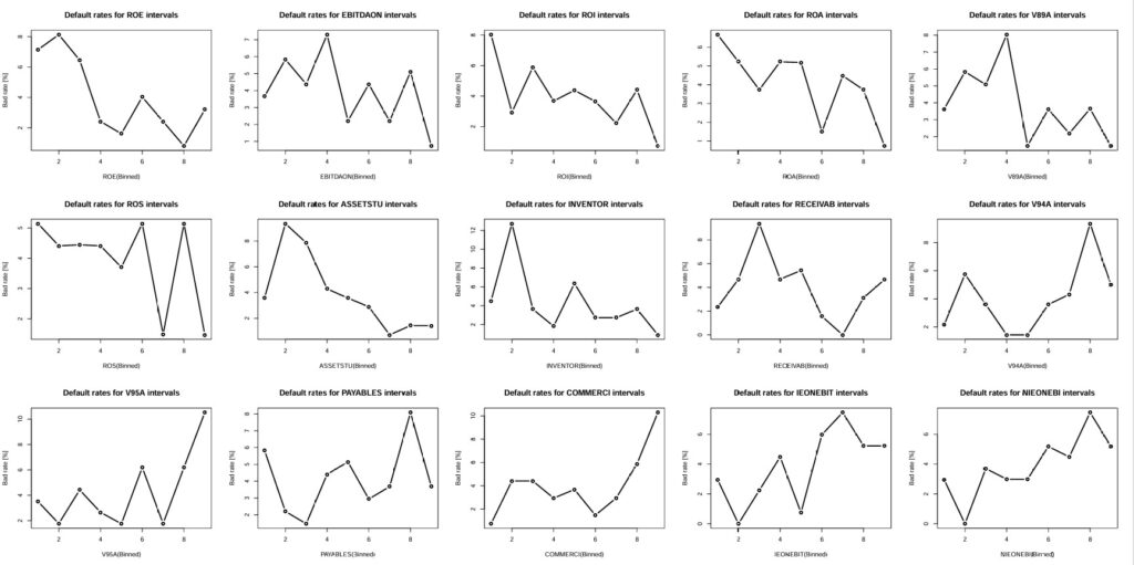
This table has the variable STATUS in first column followed by the 31 “binned” variables. We finally generate out of this table presenting the default rates for 15 variables at time
# 15 figures arranged in 3 rows and 5 columns attach(mtcars) par(mfrow=c(3,5)) for(i in 2:16){
R9VB <- table(RATIO9vSTATUS[,i], RATIO9vSTATUS$STATUS)
badrate <- R9VB[,1]/(R9VB[,1]+R9VB[,2])*100.0
R9VB <- cbind(R9VB, badrate)
plot(R9VB[,3], main = sprintf(“Default rates for %s intervals”,names(RATIO9vSTATUS)[i]), xlab = sprintf(“%s(Binned)”,names(RATIO9vSTATUS)[i]), ylab=”Bad rate [%]”)
lines(R9VB[,3], type=”b”, pch=21, col=”black”, yaxt=”n”, lwd=2)
}
Default rates variation for variables: ROE,EBITDAON,ROI,ROA,V89A,ROS,ASSETSTU,INVENTOR,RECEIVAB,V94A,V95A,PAYABLES,COMMERCI,IEONEBIT,NIEONEBI (Table_4_26_Page 178_C2_Pt1.pdf)
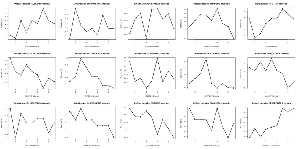
Default rates variation for variables: IEONLIAB,IEONFINA.,EXTRIC,TAXESONG,INTANGIB,TRADERE.,V110A,EQUITYON,TRADEPA.,DEBTEQU,CURRENT,QUICKRA,SALESONV,SALESMIN,ROAMINUS,EBITDAIE,EQUILIABL,DEBTEQUTR (Table_4_26_Page 178_C2_Pt2.pdf)
Default rates variation for variable: ROETR (Table_4_26_Page 178_C2_Pt3.pdf)

The results of evaluation are placed in the column “Empirical Monotinicity” from the synoptic table: Ratios_Synoptic_De Laurentis.xls Our evaluation is often in synch with that of the author.
Illustrated in Empirical Monotinicity column in the table: Ratios_Synoptic_De Laurentis.jpg
Our evaluation is often in synch with that of the author.