Step 12 – Linear Discriminant Analysis – Initial approach

PostedApril 6, 2025

UpdatedApril 6, 2025

Bywpusername7953

Purpose

Here we follow step by step the contents of Chap. 4, section 4.6.2 : Linear discriminant analysis, pp. 185-210

The authors are proposing to use Linear Discriminant Analysis method (LDA) in order to solve the problem of estimating the Probability of Default (PD) of a paticular company using its financial accounts. Like most of the Machine learning (ML) methods it is conducted in two phases:

A training phase which determines the statistical characteristics of a representative sample of both GOOD (idem, stable) companies and BD (idem, having defaulted companies). The parameters of the ML model are then determined from these characteristics.
An application (or prediction phase) when the model is used in order to predict the Probability of Default (PD) of any other company over a period which is generally the next year

In the case of Linear Discriminant Analysis method (LDA):

The training phase is conducted in two steps:
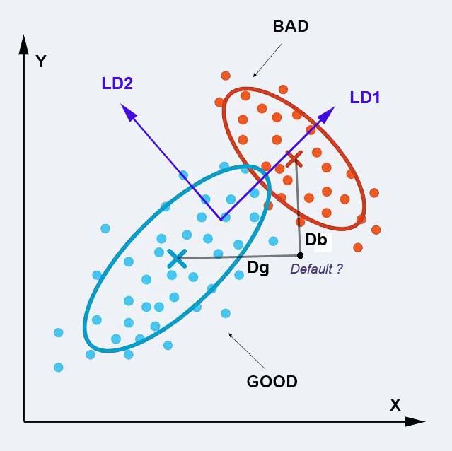
1. Each group is characterized by its average vector (or center of gravity) M and its matrix of variane-covariance Σ
2. The LDA algorithm determines a new set of coordinates which maximises the separability between groups. (In the illustration below, we go from original dimensions to new LD1,LD2 dimensions)
The prediction phase is also conducted in two steps:
1. The Mahalanobis distance between a new company X and the center of a particular group is determined as : D = (X – M)^t * Σ^-1 * (X – M). In our case, two distances are computed: Dg (GOOD) and Db (BAD)
2. The new company is then assigned to the closest group. The Mahalanobis distance being the square root of the negative Log likelihood, the probabilty (idem, likelihood) of a company to belong to this group is computed as: p = 1/₂ * e^-D2 Its is taken as the Probability of Default (PD)

IMPORTANT NOTE: The whole LDA method is based on the hypothetis that the variables (here, ratios) are Normally distributed

The principles of Linear Discriminant Analysis (LDA)

NOTE: In the present problem, we have 34 ratios (dimensions) in our data space. The dataset is composed of 1221 GOOD companies and 52 BAD companies.
For comparison, in the initial work from Altman which led to the well kwown Z-score: Altman, E.I., 1968. Financial ratios, discriminant analysis and the prediction of corporate bankruptcy. The journal of finance, 23(4), pp.589-609. https://www.jstor.org/stable/2978933
the author used 5 ratios with a balanced training data set of 33 GOOD companies and 33 BAD companies.

Method

Data preparation – -> (https://github.com/MoiraCorp/DLMM-IRating-in-R/tree/main/steps/step12/dataprep)
First run LDA on original data – -> (https://github.com/MoiraCorp/DLMM-IRating-in-R/tree/main/steps/step12/firstorgdat)
LDA on decorrelated variables using a prior PCA – -> (https://github.com/MoiraCorp/DLMM-IRating-in-R/tree/main/steps/step12/priorpca)
LDA on full author’s datatable – -> (https://github.com/MoiraCorp/DLMM-IRating-in-R/tree/main/steps/step12/fullauthdat)

Data preparation

At this point, we have the following datasets to work with:

- wcs2train the original datatable where column wcs2train$BADGOOD contains the GOOD-BAD (or default) company category
- wcs2train.ratios is a datable extracted from wcs2train and restricted to the Ratio Variables of ranks 86 to 119 in the wcs2train table
- wcs2train.ratios.NA is the wcs2train.ratios datatable where "extreme" outliers values have been turned into NAs
- wcs2train.ratios.CT is the wcs2train.ratios.NA datable where NAs have been interpolated
- wcs2train.ratios.MON is the wcs2train.ratios.NA datatable where overabundant 0s and 1s in INVENTOR, V95A and V110A have been turned into NAs

Most of the processing functions that we will be using will require that one datatable be generated were the BADGOOD vector be appended to the datatable. Ex: wcs2trainL <- cbind(wcs2train$BADGOOD, wcs2train.ratios)

In order to compare method results on an objective ground, one needs also to process the same datatable as the authors From Page 188, the authors signal that they are using the datatable: W_CS_1_AnalysisSampleDataSet_8MDA.sav

library(haven) wcs2train8MDA <- read_sav(“C:/Projets_En_Cours/AI_MTPL/UCI_Internal_Ratings/SPSS-PASW/W_CS_1_AnalysisSampleDataSet_8MDA.sav “) write.csv(wcs2train8MDA, file = “C:/Projets_En_Cours/AI_MTPL/UCI_Internal_Ratings/SPSS-PASW/ W_CS_1_AnalysisSampleDataSet_8MDA.csv”)

After this operation, the file has been re-loaded after shortening the variable names following our conventions:

wcs8trainMDA <- read.csv(“C:/Projets_En_Cours/AI_MTPL/UCI_MTPL_Internal_Ratings/SPSS-PASW/W_CS_1_AnalysisSampleDataSet_8MDA.csv”, header=TRUE, sep=”,”)

We then proceed to the extraction of the Ratio Variables and their “binned” transformations following the list proposed by the author on page 185, namely: ROE to ROETR3A and T2ROE, OVERSECT430_614, SALESBin2cl1 SALESBin2cl2
However, the xx3A variables are similar to our wcs2train.ratios.CT and they should not be left in the datatable because they are 95% redundant with the original Ratio Variables

This translates into the following list of indexes: 86:154, 156, 158, 161, 162 to which we add column 2 which contains the BADGOOD variable

vars <- c(2, 86:154, 156, 158, 161, 162) wcs8train.vars <- wcs8trainMDA[vars]

IMPORTANT NOTE : In our case, in the datatable, there is a large difference in population between GOOD Class = 1221 and the BAD class = 51 (Population total = 1272) This would give for each class and “a priori” probalility of p(GOOD) = 0.96 and p(BAD) = 0.04 (a factor of 24 !) The LDA method as well as the LOGIT method are based on the Bayes Decision rule which assigns companies on the basis of p(C)*p(C/whole population) This type of formula should make use og p(GOOD) abd P(BAD) taken from the “observed” population

HOWEVER, in pratice, much better results are obtained in LDA when “a priori” probabilities have been made equal (idem, p(GOOD)=p(BAD)=0.5)

In the following steps we are going to evaluate the improvements introduced by pre-processing the data (wcs2train.ratios, wcs2train.ratios.CT, wcs2train.ratios.MON) and will compare the results with those obtained with the final encoding porposed by the author in the wcs8trainMDA datatable;.

First run LDA on original data

Running LDA with “a priori” probabilities deduced from the size of the GOOD-BAD classes in the “observed” population

We use the cbind() and lda() functions from the MASS R package -> https://cran.r-project.org/web/packages/MASS/index.html

library(MASS) wcs2trainL <- cbind(wcs2train$BADGOOD, wcs2train.ratios) names(wcs2trainL)[1] = “BADGOOD”

NOTE: We eliminate companies (idem, rows) with NA values.

By default, the “a priori” probalities are proportional to the number of GOOD and BAD in the input datatable. We select option: CV = TRUE in oredre to perform one-off classification on each of the companies after model determination

w <- na.omit(wcs2trainL) z <- lda(BADGOOD ~ ., data=w, CV = TRUE) Warning message: In lda.default(x, grouping, …) : variables are collinear tab <- table(w$BADGOOD, z$class) tab

The printed output is:

	“Bad”	“Good”
“Bad”	2	49
“Good”	4	1212

NOTE: The LDA signals that a certain number of variables are colinear

Running LDA with equal “a priori” probabilities

The “a priori” probabilities are specified in the list: prior = c(1,1)/2

w <- na.omit(wcs2trainL) z <- lda(BADGOOD ~ ., data=w, prior = c(1,1)/2, CV = TRUE) Warning message: In lda.default(x, grouping, …) : variables are collinear tab <- table(w$BADGOOD, z$class) tab

The printed output is:

	“Bad”	“Good”
“Bad”	7	44
“Good”	146	1070

NOTE: One can witness an IMPROVEMENT when using EQUAL “A PRIORI” PROBABILITIES

LDA on decorrelated variables using a prior PCA

We start by performing a Principal Componenet Analysis (PCA) on the training data table:

library(stats) w <- na.omit(wcs2train.ratios) # Performing a Principal Component Analysis (PCA) pca <- prcomp(w, center = TRUE, scale = TRUE) # Building the data table for the LDA on PCA components. w.proj <- predict(pca, newdata=w) # Setting the number of PCA components to be used nbpcacomp = 7 varcount = 0 for(i in 1:nbpcacomp){ varcount = varcount + 1 if(varcount == 1){ varlist <- c(paste(“PC”, varcount, sep=””)) } else { varlist <- append(varlist, paste(“PC”, varcount, sep=””)) } }

Then, we project the data vectors onto the first PCA componenets and perform LDA on this one dimensional dataset.

# Selecting the first nbpcacomp PCA components w.pca <- subset(as.data.frame(w.proj),select=varlist) w <- na.omit(wcs2trainL) wcs2train.pcaL <- cbind(w$BADGOOD, w.pca) names(wcs2train.pcaL)[1] = “BADGOOD” z <- lda(BADGOOD ~ ., data=wcs2train.pcaL, prior = c(1,1)/2, CV = TRUE) table(wcs2train.pcaL$BADGOOD, z$class)

The printed output is:

	“Bad”	“Good”
“Bad”	5	46
“Good”	66	1150

NOTE: AN IMPROVEMENT IS NOTED. For class BAD, the results are very similar to those obtained with the raw data BUT for GOOD class, much less companies are misclassified

LDA on full author’s datatable

The table wcs8train.vars contains the complete data set over all the ratios

NOTE : IMPORTANT: The variable TAXESONG3A IS CONSTANT = 0 thus it must be removed before performing the LDA. This variable is situated at index = 55

library(MASS) w <- na.omit(wcs8train.vars[c(1:54,56:74)]) z <- lda(BADGOOD ~ ., data=w, prior = c(1,1)/2, CV = TRUE) Warning message: In lda.default(x, grouping, …) : variables are collinear table(w$BADGOOD, z$class)

The printed output is:

	“Bad”	“Good”
“Bad”	19	32
“Good”	162	1054

NOTE : This result is SIMILAR to the one obtained by the author using Stepwise LDA determined formula

Company Default prediction - DLMM Internal Rating Model in R

Step 12 – Linear Discriminant Analysis – Initial approach

Purpose

Method

Data preparation

First run LDA on original data

Running LDA with “a priori” probabilities deduced from the size of the GOOD-BAD classes in the “observed” population

Running LDA with equal “a priori” probabilities

LDA on decorrelated variables using a prior PCA

LDA on full author’s datatable