Company Default prediction - DLMM Internal Rating Model in R
- Steps followed to implement the DLMM Model in R language
- Step 1 – Converting SPSS formatted data
- Step 2 - One by one empirical analysis of variables
- Step 3 - Cross-tabulation 01STATUS versus Industry Sector Code
- Step 4 - Exploring graphically the probability distribution of a variable
- Step 5 - Testing the normality of the probability distribution of a variable
- Step 6 - Evaluating the good/bad discriminant power of a variable
- Step 7 - Empirical monotonicity of ROE relative to good-bad progression
- Step 8 - Correlation between variable couples
- Step 9 - Analysis of outliers
- Step 10 - Data encoding
- Step 11 - Synoptic table of variable properties
- Step 12 - Linear Discriminant Analysis - Initial approach
- Step 13 - Experimenting with Stepwise Linear Discriminant Analysis
- Step 14 - Gaussian Copula encoding scheme
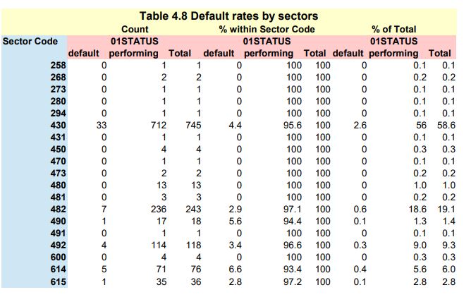
Step 3 – Cross-tabulation 01STATUS versus Industry Sector Code
It follows the section: 4.5.2 Empirical assessment of working hypothesis (page 144 of the DLMM book)
We want to compute a cross-table between the 01STATUS variable and the Industry Sector Code
in order to visualise the possible influence of the Sector of activity of a company upon its probabibilty of being in default
We use the standard table() R function for performing the cross-tabulations
Building the cross tabulation
Relating to Benzecri tensor notations, the table on page 138 is a side by side juxtaposition of:
pij, pij/pi., pij/pj. or more simply: pij, pij/pi, pij/pj
Where i (lines or rows) are SECTOR (Sector Code) and j (columns) are BADGOOD (bad/good or default/non default)
In the preceding notations, pi. and pj. are the rows and columns marginal frequencies
Starting by building the cross-table structure
cTab <- table(wcs2train$SECTOR, wcs2train$BADGOOD)
Extracting the marginal distributions
cTabi <- prop.table(cTab, 1)
cTabj <- prop.table(cTab)
Relating to Benzécri notation, cTabi is pij/pi and cTabj is pij/pj
Each of these table() objects need to be converted into dataframes for later concatenation
cTabdf <- as.data.frame.matrix(cTab)
cTabidf <- as.data.frame.matrix(cTabi)
cTabjdf <- as.data.frame.matrix(cTabj)
Adding a “total sum” column to each of these marginal tables
cTabdf$total <- cTabdf[,1] + cTabdf[,2]
cTabidf$total <- cTabidf[,1] + cTabidf[,2]
cTabjdf$total <- cTabjdf[,1] + cTabjdf[,2]
Multiplying by 100.0 the last 2 tables in order to conform to the DLMM book text and reduce the numeric format to one decimal after decimal point
indx <- sapply(cTabidf, is.numeric)
cTabidf[indx] <- lapply(cTabidf[indx], function(x) x100.0)
cTabidf[indx] <- lapply(cTabidf[indx], function(x) format(round(x, 1), nsmall = 1))
indx <- sapply(cTabjdf, is.numeric)
cTabjdf[indx] <- lapply(cTabjdf[indx], function(x) x100.0)
cTabjdf[indx] <- lapply(cTabjdf[indx], function(x) format(round(x, 1), nsmall = 1))
Row names(here: Sector Code) need to be added as a new column to these dataframes before concatenation
names <- rownames(cTabdf)
cTabr <- cbind(names, cTabdf)
cTabir <- cbind(names, cTabidf)
cTabwi <- merge(cTabr, cTabir, by=”names”)
cTabjr <- cbind(names, cTabjdf)
cTabwij <- merge(cTabwi, cTabjr, by=”names”)
The resulting table is exported to a .csv file
write.csv(cTabwij, file = “C:/Projets_En_Cours/AI_MTPL/UCI_Internal_Ratings/R Notes/defaultrates_sector.csv”)