
Company Default prediction - DLMM Internal Rating Model in R
- Steps followed to implement the DLMM Model in R language
- Step 1 – Converting SPSS formatted data
- Step 2 - One by one empirical analysis of variables
- Step 3 - Cross-tabulation 01STATUS versus Industry Sector Code
- Step 4 - Exploring graphically the probability distribution of a variable
- Step 5 - Testing the normality of the probability distribution of a variable
- Step 6 - Evaluating the good/bad discriminant power of a variable
- Step 7 - Empirical monotonicity of ROE relative to good-bad progression
- Step 8 - Correlation between variable couples
- Step 9 - Analysis of outliers
- Step 10 - Data encoding
- Step 11 - Synoptic table of variable properties
- Step 12 - Linear Discriminant Analysis - Initial approach
- Step 13 - Experimenting with Stepwise Linear Discriminant Analysis
- Step 14 - Gaussian Copula encoding scheme
Step 2 – One by one empirical analysis of variables
It follows the section: 4.5.2 Empirical assessment of working hypothesis (page 133 of the DLMM book)
We want to compute the “descriptive statistics” for each good/bad group for each of the following variables :
- ROE (Ratio Net Profit/Equity)
- IEONLIAB (Ratio Interest Expenses/Liabilities [%])
- V110A (Ratio Inventories/Total Assets [%])
We use the package “psych” in R (it is usually avalaible in the standard installation of R?) https://cran.r-project.org/web/packages/psych/psych.pdf
In this package we use function describeBy() in order to provides variable basic statistics for each of the “bad” and “good” classes
Each variable basic statistics table is saved in a separate .csv file
Loading the “psych” package
library(psych)
Computing basic good-bad satistics for variable: ROE (Ratio Net Profit/Equity)
mt_dat <- describeBy(wcs2train$ROE, wcs2train$BADGOOD, mat=T)
write.csv(mt_dat, file = “C:/Projets_En_Cours/AI_MTPL/UCI_Internal_Ratings/R Notes/describe_ROE.csv”)
mt_dat
The last command generates the following output:
item group1 vars n mean sd median trimmed mad min max range skew kurtosis se
X11 1 “Bad” 1 51 418.88892 2537.3339 0.487 6.87900 24.78907 -525 17930 18455 6.456552 41.49815 355.2978
X12 2 “Good” 1 1221 45.73707 459.6099 10.000 17.53419 31.45188 -5500 8300 13800 5.809446 139.28237 13.1532
Computing basic good-bad satistics for variable: IEONLIAB (Ratio Interest Expenses/Liabilities [%])
mt_dat <- describeBy(wcs2train$IEONLIAB, wcs2train$BADGOOD, mat=T)
write.csv(mt_dat, file = “C:/Projets_En_Cours/AI_MTPL/UCI_Internal_Ratings/R Notes/describe_IEONLIAB.csv”)
mt_dat
The last command generates the following output:
item group1 vars n mean sd median trimmed mad min max range skew kurtosis se
X11 1 “Bad” 1 51 6.487020 14.562831 4.524 4.421317 2.244656 0 107.407 107.407 6.516170 42.225823 2.03920416
X12 2 “Good” 1 1221 3.820161 2.567423 3.480 3.604277 2.379573 0 23.950 23.950 1.293554 4.471053 0.07347501
Computing basic good-bad satistics for variable: V110A (Ratio Inventories/Total Assets [%])
mt_dat <- describeBy(wcs2train$V110A, wcs2train$BADGOOD, mat=T) write.csv(mt_dat, file = “C:/Projets_En_Cours/AI_MTPL/UCI_Internal_Ratings/R Notes/describe_V110A.csv”)
mt_dat
The last command generates the following output:
item group1 vars n mean sd median trimmed mad min max range skew kurtosis se
X11 1 “Bad” 1 51 26.91231 23.82903 22.537 23.82188 20.9521 0 95.888 95.888 1.034288 0.5017606 3.3367317
X12 2 “Good” 1 1221 20.85190 23.25327 12.832 16.66432 17.5955 0 101.529 101.529 1.421104 1.4549385 0.6654664
Compare with corresponding results presented in DLMM Book
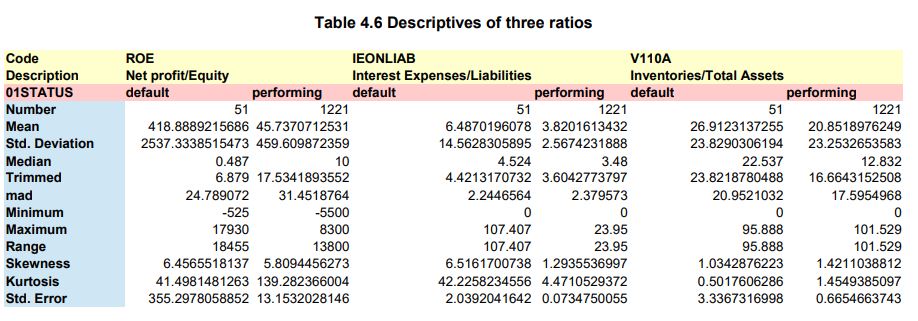
NOTE : The “pretty” presentation of the variable statistics was created by collating the 3 .csv tables in one .xls table using Edit-Paste Special-Tanspose in OpenOfficeCalc
Also, correct printing to pdf in “Lanscape” mode was set using the File-Page Preview option
The descriptive statistics match those presented in page 133 of the DLMM book.
NOTE : The last term (“se”) listed by the describeBy() function is what is called the Standard Error of the mean as explained in page 132 of the DLMM book.