
Company Default prediction - DLMM Internal Rating Model in R
- Steps followed to implement the DLMM Model in R language
- Step 1 – Converting SPSS formatted data
- Step 2 - One by one empirical analysis of variables
- Step 3 - Cross-tabulation 01STATUS versus Industry Sector Code
- Step 4 - Exploring graphically the probability distribution of a variable
- Step 5 - Testing the normality of the probability distribution of a variable
- Step 6 - Evaluating the good/bad discriminant power of a variable
- Step 7 - Empirical monotonicity of ROE relative to good-bad progression
- Step 8 - Correlation between variable couples
- Step 9 - Analysis of outliers
- Step 10 - Data encoding
- Step 11 - Synoptic table of variable properties
- Step 12 - Linear Discriminant Analysis - Initial approach
- Step 13 - Experimenting with Stepwise Linear Discriminant Analysis
- Step 14 - Gaussian Copula encoding scheme
Step 8 – Correlation between variable couples
Purpose
This implementation follows step by step the content of Chap. 4, section 4.5.7 : Correlations, pp. 160-162
Method
Testing on selected ratio variables (page 161) – -> (https://github.com/MoiraCorp/DLMM-IRating-in-R/tree/main/steps/step8/selectvar)
Correlation study for all ratio variables (page 162) – -> (https://github.com/MoiraCorp/DLMM-IRating-in-R/tree/main/steps/step8/allvar)
Using another correlation display from R – -> (https://github.com/MoiraCorp/DLMM-IRating-in-R/tree/main/steps/step8/alternr)
Testing on selected ratio variables (page 161)
In order to illustrate the process (Table 4.19, pp 161), the authors have selected the following ratio variables:
ROE-86 = Ratio Net Profit/Equity
IEONLIAB-101 = Interest Expenses/Liabilities
V110A-107 = Inventories/Total Assets
Using the cor() function from the standard R package:
The printed output is:corrprs<- cor(wcs2train[,c(86,101,107)], use=”pairwise”, method=”pearson”) corrprs
| ROE | IEONLIAB | V110A | |
|---|---|---|---|
| ROE | 1.00000000 | -0.02538354 | -0.03441025 |
| IEONLIAB | -0.02538354 | 1.00000000 | -0.03018398 |
| V110A | -0.03441025 | -0.03018398 | 1.00000000 |
In order to compute the matrix of p-value, the custom cor.pvalue() R function is used following: -> http://www.sthda.com/english/wiki/visualize-correlation-matrix-using-correlogram
cor.pvalue <- function(mat, …) { mat <- as.matrix(mat) n <- ncol(mat) p.mat<- matrix(NA, n, n) diag(p.mat) <- 0 for (i in 1:(n – 1)) { for (j in (i + 1):n) { tmp <- cor.test(mat[, i], mat[, j], …) p.mat[i, j] <- p.mat[j, i] <- tmp$p.value } } colnames(p.mat) <- rownames(p.mat) <- colnames(mat) p.mat }
The printed output is:# matrix of the p-value of the correlation p.mat<- cor.pvalue (wcs2train[,c(86,101,107)]) p.mat
| ROE | IEONLIAB | V110A | |
|---|---|---|---|
| ROE | 0.0000000 | 0.3656972 | 0.2200474 |
| IEONLIAB | 0.3656972 | 0.0000000 | 0.2820608 |
| V110A | 0.2200474 | 0.2820608 | 0.0000000 |
The printed output is:corrspm<- cor(wcs2train[,c(86,101,107)], use=”pairwise”, method=”spearman”) corrspm
| ROE | IEONLIAB | V110A | |
|---|---|---|---|
| ROE | 1.00000000 | -0.15264427 | -0.05102912 |
| IEONLIAB | -0.15264427 | 1.00000000 | 0.02129009 |
| V110A | -0.05102912 | 0.02129009 | 1.00000000 |
In supplement, the R cor() function offers the Kendall parametric correlation
The printed output is:corrken<- cor(wcs2train[,c(86,101,107)], use=”pairwise”, method=”kendall”) corrken
| ROE | IEONLIAB | V110A | |
|---|---|---|---|
| ROE | 1.0000000 | -0.10461972 | -0.03484200 |
| IEONLIAB | -0.1046197 | 1.00000000 | 0.01552111 |
| V110A | -0.0348420 | 0.01552111 | 1.00000000 |
Correlation study for all ratio variables (page 162)
The ratio variables span indexes 86 to 119 in the 7a) Testing on selected ratio variables (page 161) data table
We are using the corrplot R package for display.<br We are following the examples of: -> http://www.sthda.com/english/wiki/visualize-correlation-matrix-using-correlogram
install.packages(“corrplot”)
library(corrplot)
corrprs <- cor(wcs2train[,c(86:119)], use=”pairwise”, method=”pearson”)
p.mat <- cor.pvalue(wcs2train[,c(86:119)])
col <- colorRampPalette(c(“#BB4444”, “#fcc3b8”, “#FFFFFF”, “#add2f7”, “#4fc69d”))
corrplot(corrprs, method=”color”, col=col(200),
type=”upper”,
addCoef.col = “black”, # Add coefficient of correlation
addCoefasPercent = TRUE,
tl.col=”black”, tl.srt=45, # Text label color and rotation
# Combine with significance p.mat = p.mat, sig.level = 0.01, insig = “blank”,
# hide correlation coefficient on the principal diagonal
diag=FALSE
)
NOTE: Hexa ramp colors have been tuned using tool in Google Search. The display blanks out the color of cells below significance level of 0.01 (1%), as indicated on page 160, last line.
The graphics representation of the Pearson correlation between all Ratio Variables is presented in: Table_4_19b_Page 162_Ratios_Correlation.pdf
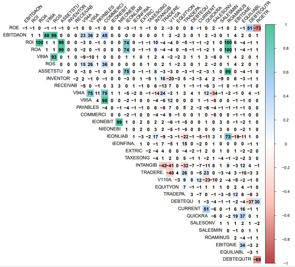
From this diagram, we detremine the following groups of correlated variables (over 70%).
NOTE: The groups are identical to those proposed in the author’s text
GR1: ROE, ROETR (Negative 73% with ROE), DEBTEQUTR (Negative 69% with ROETR and 51% with ROE)
| Column in R table | Code in text | Description |
|---|---|---|
| ROE-86 | ROE | Ratio Net Profit/Equity |
| DEBTEQUTR-118 | DebtEquityTr | Ratio Interest-bearing Financial Debt/Equity |
| ROETR-119 | ROETr | Ratio Net Profit/Total Stockholder’s Equity |
GR2: EBITDAON, V89A (88% with EBITDAON), ROS (99% with EBITDAON)
| Column in R table | Code in text | Description |
|---|---|---|
| EBITDAON-87 | EBITDAonSALES | Ratio EBITDA/Sales [%] |
| V89A-90 | EBITDAonVP | Ratio EBITDA/Value of Production |
| ROS-91 | ROS | Ratio EBIT/Sales [%] |
GR3: ROI, ASSETSTU (99% with ROI and ROA), ROA (100% with ROI), IEONLIAB (73% with ROAMINUS), ROAMINUS (100% with ROI and ROA and 99% with ASSETSTU)
| Column in R table | Code in text | Description |
|---|---|---|
| ROI-88 | ROI | Ratio EBIT/Operating Assets [%] |
| ASSETSTU-92 | ASSETS_TURNOVER | Ratio Total Assets/Turnover |
| ROA-89 | ROA | Ratio Current Income/Total Assets [%] |
| IEONLIAB-101 | IEonLIABLITIES | Ratio Interest Expenses/Liabilities [%] |
| ROAMINUS-115 | ROAminusIEonTL | ROA minus Ratio Interest Expenses/Total Liabilities |
GR4: V94A, V95A, COMMERCI (98% with V95A)
| Column in R table | Code in text | Description |
|---|---|---|
| V94A-95 | RECEIVABLES_PERIOD | Ratio Trade Receivables/Daily Sales |
| V95A-96 | INVENTORY_PERIOD | Ratio Inventory/Daily Sales |
| COMMERCI-98 | COMMERCIAL_WC_PERIOD | Ratio (Trade Receivables + Inventory – Trade Payables)/Daily Sales |
GR5: IEONEBIT, NIEONEBI (99%)
| Column in R table | Code in text | Description |
|---|---|---|
| IEONEBIT-99 | IEonEBITDA | Ratio Interest Expenses/EBITDA [%] |
| NIEONEBI-100 | NIEonEBITDA | Ratio Net Interest Expenses/EBITDA [%] |
This kind of display display gives a “direct” impression of the bi-variate cloud points.
It uses the chart.Correlation() function from the PerformanceAnalytics R package -> https://cran.r-project.org/web/packages/PerformanceAnalytics/index.html
chart.Correlation(wcs2train[,c(86:119)], histogram=TRUE, pch=19)
Illustrated in Table_4_19d_Page162_Allvariables_CoorDiag.pdf
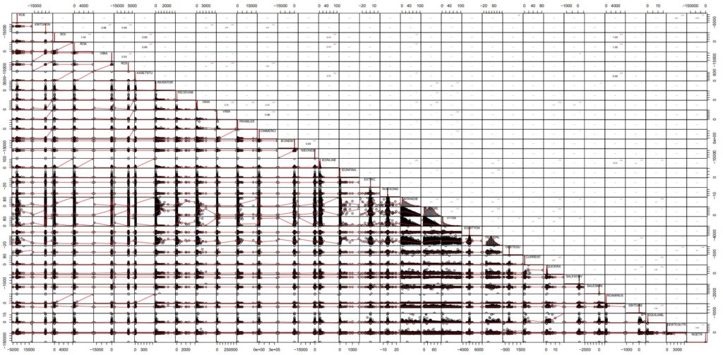
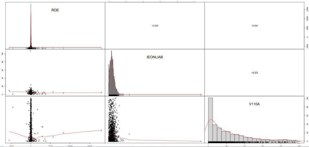
NOTE : From this display, it is apparent that “outliers” play an important role in the charactersization of correlation properties, in particaular in the case of ROE. The subject of “outliers” is dealt with in the next section.