
Company Default prediction - DLMM Internal Rating Model in R
- Steps followed to implement the DLMM Model in R language
- Step 1 – Converting SPSS formatted data
- Step 2 - One by one empirical analysis of variables
- Step 3 - Cross-tabulation 01STATUS versus Industry Sector Code
- Step 4 - Exploring graphically the probability distribution of a variable
- Step 5 - Testing the normality of the probability distribution of a variable
- Step 6 - Evaluating the good/bad discriminant power of a variable
- Step 7 - Empirical monotonicity of ROE relative to good-bad progression
- Step 8 - Correlation between variable couples
- Step 9 - Analysis of outliers
- Step 10 - Data encoding
- Step 11 - Synoptic table of variable properties
- Step 12 - Linear Discriminant Analysis - Initial approach
- Step 13 - Experimenting with Stepwise Linear Discriminant Analysis
- Step 14 - Gaussian Copula encoding scheme
Step 7 – Empirical monotonicity of ROE relative to good-bad progression
Purpose
This implementation follows step by step the content of Chap. 4, section 4.5.6 : Empirical monotonicity, pp. 157-160
Method
Comparison between BADGOOD distribution and a binned ROE – -> (https://github.com/MoiraCorp/DLMM-IRating-in-R/tree/main/steps/step7/binning)
Comparison between BADGOOD distribution and the sign of ROE numerator and denominator – -> (https://github.com/MoiraCorp/DLMM-IRating-in-R/tree/main/steps/step7/signs)
Developing a var/BADGOOD monotonicity detection scheme – -> (https://github.com/MoiraCorp/DLMM-IRating-in-R/tree/main/steps/step7/monotonicity)
Comparison between BADGOOD distribution and a binned ROE
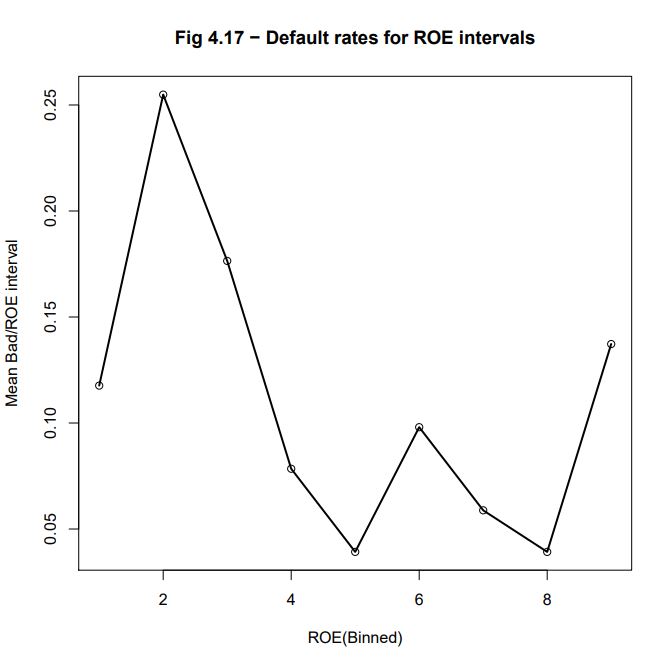
The authors state that “empirical motonicity” between a (continuous or ordinal) variable X and the BADGOOD classes happens when we obtain a monotonic increase (or decrease) of default rates (idem, relative number of “Bad” companies) relatively to variable X categorized into continuous ordered intervals (idem, encoded as an ordinal variable) In this case the comparison element is the average of default rates of borrowers included into variable X category intervals (idem, for example, the number of “Bad” companies in the interval divided by total number of these “Bad” companies)
NOTE: This “empirical motonicity” property tranlates into what is called a “Guttman Effect” in J. P. Benzécri Correspondence Analysis Theory (see: J-P Benzécri, Correspondence Analysis Handbook, Statistics: A Series of Textbooks and Monograph series, CRC Press, 1992, 688 pages, ISBN: 0824784375 or Blasius, J. (2011). Correspondence Analysis. In: Lovric, M. (eds) International Encyclopedia of Statistical Science. Springer, Berlin, Heidelberg. https://doi.org/10.1007/978-3-642-04898-2_195)
The binning function bin.var()
We are binning the ROE variable in 9 (10 boundaries) equally populated bins using the special purpose bin.var () function developed in R
bin.var <- function (x, bins = 4, method = c(“intervals”, “proportions”, “natural”), labels = FALSE) = { method <- match.arg(method) if (length(x) < bins) { stop(“The number of bins exceeds the number of data values”) } x <- if (method == “intervals”) cut(x, bins, labels = labels) else if (method == “proportions”) cut(x, quantile(x, probs = seq(0, 1, 1/bins), na.rm = TRUE), include.lowest = TRUE, labels = labels) else { xx <- na.omit(x) breaks <- c(-Inf, tapply(xx, KMeans(xx, bins)$cluster, max))<br cut(x, breaks, labels = labels) } as.factor(x) }
Building an encoded ROE into 9 equal-population intervals (10 boundaries)
Listing the boundaries of the encoding
The printed output is:bins_cut = 9 quant <- quantile(wcs2train$ROE, probs = seq(0, 1, 1/bins_cut), na.rm = TRUE) quant
0% 11.11111% 22.22222% 33.33333% 44.44444% 55.55556% 66.66667% 77.77778% 88.88889% 100% -5500.000000 -47.512000 -5.779667 1.370000 5.747778 13.950778 25.828667 48.020222 100.000000 17930.000000
Encoding ROE as a factor
The printed output is:bins_cut = 9 for(j in 1:bins_cut) { if(j == 1){ collist <- c(sprintf(“%s_1″,”ROE”)) } else { collist <- append(collist, sprintf(“%s_%s”,”ROE”,j)) } } ROE9 <- with(wcs2train, bin.var(wcs2train$ROE, bins=bins_cut, method=’proportions’, labels=collist)) table(ROE9, wcs2train$BADGOOD)
ROE9 “Bad” “Good” ROE_1 6 136 ROE_2 13 128 ROE_3 9 133 ROE_4 4 136 ROE_5 2 139 ROE_6 5 136 ROE_7 3 138 ROE_8 2 141 ROE_9 7 133
Graphing the binned ROE
plot(ROE9VB[,1], main = “Fig 4.17 – Default rates for ROE intervals”, xlab=”ROE(Binned)”, ylab=”Mean Bad/ROE interval”) lines(ROE9VB[,1], lwd=2)
The resulting graph is presented in : Fig_4_17_Page 158_ROEBin_Bad.pdf
Comparison between BADGOOD distribution and the sign of ROE numerator and denominator
In the W_CS_1_AnalysisSampleDataSet_2B.xls database: ROE-86 = NPROF-85 / EQUITY-29
We are using the describe() function from the R psych package -> https://cran.r-project.org/web/packages/psych/index.html in order obtain descriptive statistics for each of the variables of the wcs2train (Version 2B) table.
library(psych) deswcs2train_2B <- describe(wcs2train) write.csv(deswcs2train_2B, file = “C:/Projets_En_Cours/AI_MTPL/UCI_Internal_Ratings/R Notes/deswcs2train_2B.csv”)
The available statistics gerneratd by the describe function are:
- vars: index of variable in table
- n: number of valid members (except for NA)
- mean: mean or average
- sd: standard deviation
- median: median
- trimmed: trimmed mean (with trim defaulting to .1) ?
- mad: median absolute deviation (from the median)
- min: minimum value
- max: maximum value
- range: range length
- skew: skew
- kurtosis: kurtosis
- se: r.m.s. error
For NPROF-85 and EQUITY-29 we get the following printed results:
var		min		max		range
NPROF-85	-5379		5327		10706
EQUITY-29	-3685		152567		156252
The printed output is:NPROFsign <- cut(wcs2train$NPROF, breaks=c(-Inf, -1, 0, Inf), labels=c(“-“, “0”, “+”), include.lowest=FALSE) summary(NPROFsign)
-	0	+
230	16	1025
The printed output is:EQUITYsign <- cut(wcs2train$EQUITY, breaks=c(-Inf, -1, 0, Inf), labels=c(“-“, “0”, “+”), include.lowest=FALSE) summary(EQUITYsign)
- 	0 	+
200	6 	1065
The printed output is:STATUS <- wcs2train$BADGOOD ROEsign <- cbind(STATUS=levels(STATUS)[STATUS], NPROFsign=levels(NPROFsign)[NPROFsign], EQUITYsign=levels(EQUITYsign)[EQUITYsign]) summary(ROEsign)
STATUS		NPROFsign	EQUITYsign
"Bad" :  51 	-: 230		-: 200
"Good":1220	+:1025		+:1065
     		0:  16    	0:   6
Building a 3-way count table mimicking that of Table 4.18, page 159
The printed output is:EQUNPRvSTATUS <- xtabs(~ EQUITYsign + NPROFsign + STATUS, ROEsign) EQUNPRvSTATUS, , STATUS = “Bad”
		NPROFsign
EQUITYsign	-	+	0
	-	4	9	0
	+	14	24	0
	0	0	0	0
The printed output is:EQUNPRvSTATUS <- xtabs(~ EQUITYsign + NPROFsign + STATUS, ROEsign) EQUNPRvSTATUS, , STATUS = “Good”
		NPROFsign
EQUITYsign	-	+	0
	-	47	138	2
	+	165	848	14
	0	0	6	0
Developing a var/BADGOOD monotonicity detection scheme
Testing MCA for detecting monotonicity
Building a data.frame ROE9vSTATUS containing the cross-table between the binned ROE9 variable (ROE binned in 9 levels) versus STATUS variable It needs to use the bin.var() function which R code has neen introduced in this exrecise in the section: step7-binning and the R FactoMineR package -> https://cran.r-project.org/web/packages/FactoMineR/index.html
The printed output is:library(FactoMineR) ROE9 <- with(wcs2train, bin.var(wcs2train$ROE, bins=bins_cut, method=’proportions’, labels=collist)) STATUS <- wcs2train$BADGOOD ROE9vSTATUS <- cbind(ROE9=levels(ROE9)[ROE9], STATUS=levels(STATUS)[STATUS]) summary(ROE9vSTATUS)
ROE9 STATUS ROE_8 :143 “Bad” : 51 ROE_1 :142 “Good”:1220 ROE_3 :142 ROE_2 :141 ROE_5 :141 ROE_6 :141 (Other):421
We then run the MCA (Multiple Correspondence Analysis) on the cross-table and list the factors scores on the first component
The printed output is:ROE9vSTATUS.res<-MCA(ROE9vSTATUS, ncp=2, graph = TRUE) summary(ROE9vSTATUS.res)
Categories (the 10 first) Dim.1 ROE_1 0.066 ROE_2 1.619 ROE_3 0.723 ROE_4 0.359 ROE_5 -0.807 ROE_6 -0.145 ROE_7 -0.586 ROE_8 -0.813 ROE_9 0.307
If the encoded variable ROE9 would be monotic versus STATUS (BADGOOD) then the coordinates of ROE_1 to ROE_9 on the first axis should be respect-full of the order 1 to 9 (Guttman effect) We will use this property in oreder to build a test for monotonicity which will be called “MCA Monotonicity test”
Performing the MCA monotonicity test on all the ratio variables
The test is performed on the variables recommended for their monotonicity on page 160. to the exception of V95A-96, V110A-107 for the bin.var() function does not behave appropriatley with parameters “bin.cut” and “proportions”
- EBITDAON-87 -> EBITDAonSALES = Ratio EBITDA/Sales [%]
- ROI-88 -> ROI = Ratio EBIT/Operating Assets [%]
- ASSETSTU-92 -> ASSETS_TURNOVER = Ratio Total Assets/Turnover
- PAYABLES-97 -> PAYABLES_PERIOD = Ratio Trade Payables/Daily Purchases
- IEONLIAB-101 -> IEonLIABLITIES = Ratio Interest Expenses/Liabilities [%]
- IEONFINA-102 -> IEonFINANCIAL_DEBTS = Ratio Interest Expenses/Financial Debts [%]
- TRADEPA-109 -> TRADE_PAYABLESonTL = Ratio Trade Payables/Total Liabilities [%]
- EQUITYON-108 -> EQUITYonPERMANENT_CAPITAL = Ratio Equity/Permanent Capital [%]
- ROAMINUS-115 -> ROAminusIEonTL = ROA minus Ratio Interest Expenses/Total Liabilities
The results are illustrated in: Fig_4_17b_Page 160_Ratios_BadvGood.pdf
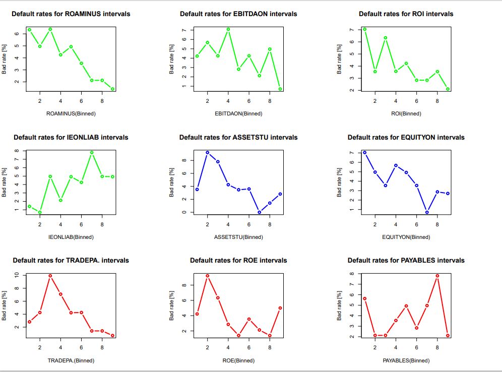
NOTE : Variables plotted in green show a “good” monotonicity, those plotted in blue are “fair” and those plotted in red are “poor” and among them is the ROE variable studied before.