
Company Default prediction - DLMM Internal Rating Model in R
- Steps followed to implement the DLMM Model in R language
- Step 1 – Converting SPSS formatted data
- Step 2 - One by one empirical analysis of variables
- Step 3 - Cross-tabulation 01STATUS versus Industry Sector Code
- Step 4 - Exploring graphically the probability distribution of a variable
- Step 5 - Testing the normality of the probability distribution of a variable
- Step 6 - Evaluating the good/bad discriminant power of a variable
- Step 7 - Empirical monotonicity of ROE relative to good-bad progression
- Step 8 - Correlation between variable couples
- Step 9 - Analysis of outliers
- Step 10 - Data encoding
- Step 11 - Synoptic table of variable properties
- Step 12 - Linear Discriminant Analysis - Initial approach
- Step 13 - Experimenting with Stepwise Linear Discriminant Analysis
- Step 14 - Gaussian Copula encoding scheme
Step 14 – Gaussian Copula encoding scheme
Purpose
The gaussian anamorphosis, known also as Gaussian Copula encoding is a mathematical function which transforms a variable X with any density distribution into a new variable Y with a Gaussian density distribution. As the Linear Discriminant Analysis method is based on the comparison between GOOD and BAD groups which variables are normaly distributed (idem, Gauss shaped density), Gaussian Copula encoding is a way to adapt the data so that it optimaly fits the LDA instrument.
This aspect of data pre-processing is addressed by the authors in section 4.5.9 Transformation of indicators (pages: 164-177). Although it is there essentially based on the use of formula based transformations and not in terms of a transformative transition between probability distributions. We have in particular evaluated the use of the LOGIT recoding function in: evaluated Step10 – Transformation of indicators using a logistic formula: the case of the ROE ratio – -> (https://github.com/MoiraCorp/DLMM-IRating-in-R/tree/main/steps/step10/logencode)
The concept of transition between two probability distributions was first formulated by J. P. Benzécri, in 1963 in his development of Correspondence Analysis as an inductive linguistics method of staistical text analysis. (see -> Benzécri, J.P., 1969. Statistical analysis as a tool to make patterns emerge from data. In Methodologies of pattern recognition (pp. 35-74). Academic Press. https://helios2.mi.parisdescartes.fr/~lerb/publications/HONOLULU.pdf)
Illlustration of Benzécri concept of probability transition nowadays often better known as “copula”
These concepts later inspired G. Matheron who had created a linear method for the interpolation of two dimensional fields known as “Kriging”. As any linear probability implies using the hypothesis of Normally distributed radom variables, G. Matheron sought to improve the perfomance of “Kriging” by applying a prior transition from observed probability distributions to Gauus shaped ones. Realizing that in practice probability transition could only be algorithmically implemented on discrete probability distributions, G. Matheron developed in 1976 both a discrete based interpolation method known as “Disjunctive kriging” and a probability transition algorithm under the name of “Gaussian Anamorphosis” (see -> Matheron, G. and Kleingeld, W.J., 1987. The evolution of geostatistics. In APCOM (Vol. 87, pp. 9-12) https://www.saimm.co.za/Conferences/Apcom87Geostatistics/009-Matheron.pdf )
Paralell to these developments, A. Sklar, introduced in 1959 the concept of “copula” which is similar to that of J.P. Benzécri probablity transition (or correspondence) (see -> “Fonctions de répartition à n dimensions et leurs marges”, Publ. Inst. Statist. Univ. Paris, 8: 229–231 https://hal.science/hal-04094463/document ). This concept has known a considerable application developement since the 1990’s, this is why we will prefer the term of Gaussian Copula encoding to that of gaussian anamorphosis because the application of the last one is restricted to the domain of geotatistics.
Exploring Gaussian Copula encoding – -> (https://github.com/MoiraCorp/DLMM-IRating-in-R/tree/main/steps/step14/gausscop)
Testing GOOD-BAD separability with Uniform and Gaussian Copula encoding – -> (https://github.com/MoiraCorp/DLMM-IRating-in-R/tree/main/steps/step14/unigausscopul)
Using Gaussian Copula encoding for LDA – -> (https://github.com/MoiraCorp/DLMM-IRating-in-R/tree/main/steps/step14/gausscoplda)
In order to transform each ratio variable so that its final distribtion is Gaussian shaped, we are using a 2 steps procedure:
- In the first step, the variable is encoded on 256 discrete intervals such as each of these intervals holds the smae amount of companies (idem, isopulation encoding)
- In the second step, a transition table is aplied to these 256 intervals so that the final encoded variable display a Gauss shaped distribution
For the second step, the transition table (name tgauss) is borrowed from the Minimimage software which was developed at CTAMN-Ecole des Mines de Paris for the the purpose of satellite image processing and released as open code written in Delphi-Pascal (see -> https://code.google.com/archive/p/teravue-16bits-delphi/ )
# The Gauss conversion table used in Minimage coiso.pas subroutine
tgauss <- c( 0, 14, 24, 31, 36, 40, 43, 46, 48, 50, 52, 54, 56, 58, 59, 61,
62, 63, 65, 66, 67, 68, 69, 70, 71, 72, 73, 74, 75, 76, 77, 78,
79, 79, 80, 81, 82, 82, 83, 84, 85, 85, 86, 87, 87, 88, 89, 89,
90, 90, 91, 92, 92, 93, 93, 94, 95, 95, 96, 96, 97, 97, 98, 98,
99, 99,100,100,101,101,102,102,103,103,104,104,105,105,106,106,
107,107,108,108,109,109,110,110,111,111,111,112,112,113,113,114,
114,115,115,115,116,116,117,117,118,118,118,119,119,120,120,121,
121,121,122,122,123,123,124,124,124,125,125,126,126,126,127,127,
128,128,129,129,129,130,130,131,131,131,132,132,133,133,134,134,
134,135,135,136,136,137,137,137,138,138,139,139,140,140,140,141,
141,142,142,143,143,144,144,144,145,145,146,146,147,147,148,148,
149,149,150,150,151,151,152,152,153,153,154,154,155,155,156,156,
157,157,158,158,159,159,160,160,161,162,162,163,163,164,165,165,
166,166,167,168,168,169,170,170,171,172,173,173,174,175,176,176,
177,178,179,180,181,182,183,184,185,186,187,188,189,190,192,193,
194,196,197,199,201,203,205,207,209,212,215,219,224,231,241,255)
For illustration, we are applying this Gaussian Copula coding schme to the ROE ratio data form the wcs2train datatable.
We are using two functions which are avilable in the standard R package:
- the quantile function (-> https://www.rdocumentation.org/packages/stats/versions/3.6.2/topics/quantile )
- the .bincode binning function (-> https://www.rdocumentation.org/packages/base/versions/3.6.2/topics/.bincode )
# Generating the isopopulation encoded variable: ROE256 bins_cut = 255 ROE256 <- .bincode(wcs2train$ROE, quantile(wcs2train$ROE, probs = seq(0, 1, 1/bins_cut), na.rm = TRUE), TRUE) # Generating the Guass Copula encoded variable: ROE256G ROE256G <- c() ROE256G <- vector(mode=”numeric”, length(ROE256)) for(i in 1:length(ROE256)){
ROE256G[i] <- tgauss[ROE256[i]+1]
}
# Producing an illustration comparing the histograms of ROE256 and ROE256G
# 2 figures arranged in 1 row and 3 columns
attach(mtcars)
par(mfrow=c(1,3))
hist(wcs2train$ROE, breaks = 50)
hist(ROE256, breaks = 50)
hist(ROE256G, breaks = 50)
Illustrated in: Histo_ROE_to_Isopulation_to_Gauss.pdf
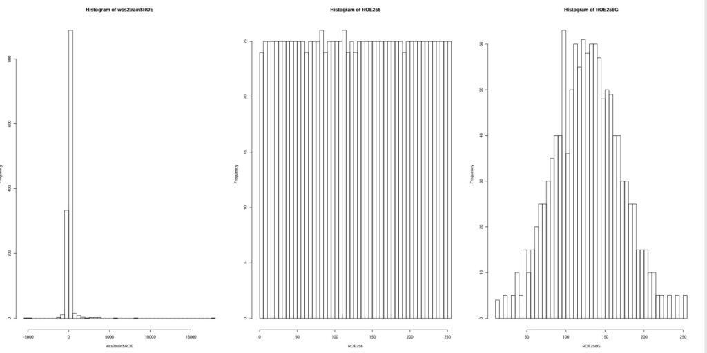
NOTE: Final results seems quite satisfactoty, comparison of ROE spread in isopopulation and with Gauss encoding.
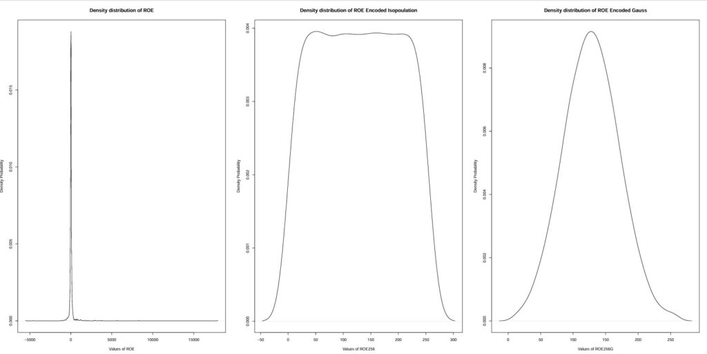
# Producing an illustration comparing the histograms of ROE256 and ROE256G
# 1 figures arranged in 1 rows and 3 columns
attach(mtcars) par(mfrow=c(1,3))
plot(density(wcs2train$ROE, na.rm=TRUE),
main = sprintf(“Density distribution of ROE”),
xlab = sprintf(“Values of ROE”), ylab=”Density Probability”)
plot(density(ROE256, na.rm=TRUE),
main = sprintf(“Density distribution of ROE Encoded Isopoulation”),
xlab = sprintf(“Values of ROE256″), ylab=”Density Probability”)
plot(density(ROE256G, na.rm=TRUE),
main = sprintf(“Density distribution of ROE Encoded Gauss”),
xlab = sprintf(“Values of ROE256G”), ylab=”Density Probability”)
For better esthetics with densities: Density_ROE_to_Isopulation_to_Gauss.pdf
We are testing the effect of the Gauss Copula encoding on the separability between BAD and GOOD groups for the ROE ratio.
library(ggplot2)
library(“gridExtra”)
my_plots = list()
# 3 figures arranged in 1 rows and 3 columns
x <- wcs2train$ROE
y <- wcs2train$BADGOOD
d <- data.frame(x,y)
my_plots[[1]] <- qplot(x, data=d, geom=”density”, fill=y, alpha=I(.5),
main = sprintf(“Density distribution of ROE”), xlab=”x”,
ylab=”Density”)
x <- ROE256
y <- wcs2train$BADGOOD
d <- data.frame(x,y)
my_plots[[2]] <- qplot(x, data=d, geom=”density”, fill=y, alpha=I(.5),
main = sprintf(“Density distribution of ROE Encoded Isopopulation”), xlab=”x”,
ylab=”Density”)
x <- ROE256G
y <- wcs2train$BADGOOD
d <- data.frame(x,y)
my_plots[[3]] <- qplot(x, data=d, geom=”density”, fill=y, alpha=I(.5),
main = sprintf(“Density distribution of ROE Encoded Gauss”), xlab=”x”,
ylab=”Density”)
grid.arrange(grobs = my_plots, nrow = 1)
Illustrated in: Separability_BAD-GOOD_ROE_to_Isopulation_to_Gauss.pdf
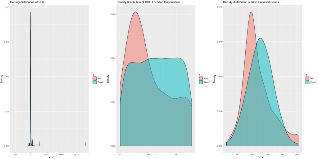
NOTE: Despite overlap, a useful and clear cutting point appears for both isopopulation and Gauss copula encoding
Using Gaussian Copula encoding for LDA
Data preparation
The printed output is:# The names of variables have been simplified according to W_CS_1_Schema.xls (Done using OpenOffice) # BADGOOD variable values have been transformed : 0 -> “Good” and 1 -> “Bad” (Done using OpenOffice) wcs9train <- read.csv(“C:/Projets_En_Cours/AI_MTPL/UCI_MTPL_Internal_Ratings/SPSS-PASW/W_CS_1_AnalysisSampleDataSet_9MDAbin.csv”, header=TRUE, sep=”,”) summary(wcs9train$BADGOOD)
| Group code | “Bad” | “Good” |
|---|---|---|
| 51 | 1221 |
Selecting DL Ratios used for model determination from ROE to ROETR
ratiovars <- c(86:119) wcs9train.ratios <- wcs9train[ratiovars] sapply(wcs9train.ratios, class) ROE EBITDAON ROI ROA V89A ROS ASSETSTU INVENTOR RECEIVAB V94A V95A PAYABLES COMMERCI IEONEBIT NIEONEBI IEONLIAB IEONFINA. EXTRIC “numeric” “numeric” “numeric” “numeric” “numeric” “numeric” “numeric” “numeric” “numeric” “numeric” “numeric” “numeric” “numeric” “numeric” “numeric” “numeric” “numeric” “numeric” TAXESONG INTANGIB TRADERE. V110A EQUITYON TRADEPA. DEBTEQU CURRENT QUICKRA SALESONV SALESMIN ROAMINUS EBITDAIE EQUILIABL DEBTEQUTR ROETR “numeric” “numeric” “numeric” “numeric” “numeric” “numeric” “numeric” “numeric” “numeric” “numeric” “numeric” “numeric” “numeric” “numeric” “numeric” “integer”
There are 34 columnsnames(wcs9train.ratios) [1] “ROE” “EBITDAON” “ROI” “ROA” “V89A” “ROS” “ASSETSTU” “INVENTOR” “RECEIVAB” “V94A” “V95A” “PAYABLES” “COMMERCI” “IEONEBIT” “NIEONEBI” [16] “IEONLIAB” “IEONFINA.” “EXTRIC” “TAXESONG” “INTANGIB” “TRADERE.” “V110A” “EQUITYON” “TRADEPA.” “DEBTEQU” “CURRENT” “QUICKRA” “SALESONV” “SALESMIN” “ROAMINUS” [31] “EBITDAIE” “EQUILIABL” “DEBTEQUTR” “ROETR”
length(wcs9train.ratios) [1] 34
Proceeding with the Gauss Copula encoding
# Loading the Gauss Copula encoding table tgauss <- c( 0, 14, 24, 31, 36, 40, 43, 46, 48, 50, 52, 54, 56, 58, 59, 61, 62, 63, 65, 66, 67, 68, 69, 70, 71, 72, 73, 74, 75, 76, 77, 78, 79, 79, 80, 81, 82, 82, 83, 84, 85, 85, 86, 87, 87, 88, 89, 89, 90, 90, 91, 92, 92, 93, 93, 94, 95, 95, 96, 96, 97, 97, 98, 98, 99, 99,100,100,101,101,102,102,103,103,104,104,105,105,106,106, 107,107,108,108,109,109,110,110,111,111,111,112,112,113,113,114, 114,115,115,115,116,116,117,117,118,118,118,119,119,120,120,121, 121,121,122,122,123,123,124,124,124,125,125,126,126,126,127,127, 128,128,129,129,129,130,130,131,131,131,132,132,133,133,134,134, 134,135,135,136,136,137,137,137,138,138,139,139,140,140,140,141, 141,142,142,143,143,144,144,144,145,145,146,146,147,147,148,148, 149,149,150,150,151,151,152,152,153,153,154,154,155,155,156,156, 157,157,158,158,159,159,160,160,161,162,162,163,163,164,165,165, 166,166,167,168,168,169,170,170,171,172,173,173,174,175,176,176, 177,178,179,180,181,182,183,184,185,186,187,188,189,190,192,193, 194,196,197,199,201,203,205,207,209,212,215,219,224,231,241,255) bins_cut = 255 # Encoding all ratios using Gauss Copula wcs9train.ratiosG <- wcs9train.ratios for(i in 1:34){ # Calling .bincode() with quantile(na.rm = TRUE) remove NA and right = TRUE, include.lowest = TRUE, thus generating 256 entries (0 to 255) rm(QUANT256) QUANT256 <- .bincode(wcs9train.ratios[,i], quantile(wcs9train.ratios[,i], probs = seq(0, 1, 1/bins_cut), na.rm = TRUE), right = TRUE, include.lowest = TRUE) for(j in 1:length(QUANT256)){ wcs9train.ratiosG[j,i] <- tgauss[QUANT256[j]] } }
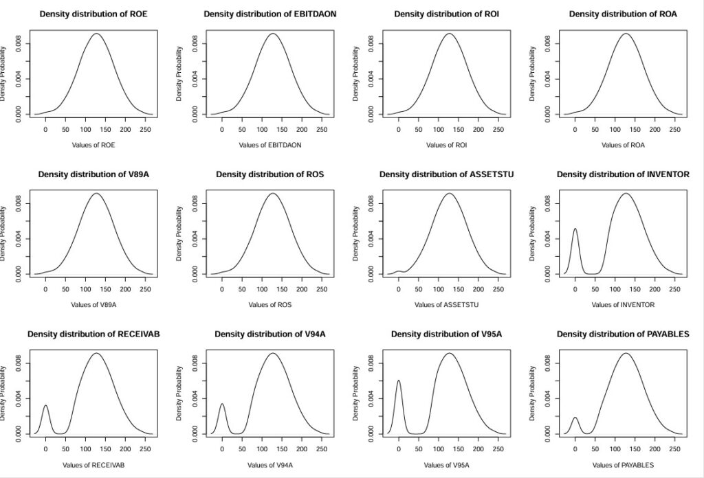
Checking on the separability of Gauss Copula encoded ratios
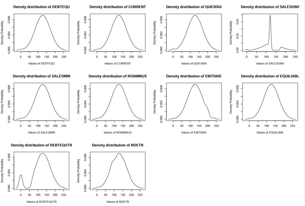
library(grid) library(gridExtra) library(ggplot2) # 12 figures arranged in 3 rows and 4 columns – Part 1 attach(mtcars) par(mfrow=c(3,4)) for(i in 25:34){ plot(density(wcs9train.ratiosG[,i], na.rm=TRUE), main = sprintf(“Density distribution of %s”,names(wcs9train.ratiosG)[i]), xlab = sprintf(“Values of %s”,names(wcs9train.ratiosG)[i]), ylab=”Density Probability”) }
Histograms for ratios: ROE,EBITDAON,ROI,ROA,V89A,ROS,ASSETSTU,INVENTOR,RECEIVAB,V94A,V95A,PAYABLES (Density_wcs9train.ratiosG-1-12.pdf)
Histograms for ratios: COMMERCI,IEONEBIT,NIEONEBI,IEONLIAB,IEONFINA.,EXTRIC,TAXESONG,INTANGIB,TRADERE.,V110A,EQUITYON,TRADEPA. (Density_wcs9train.ratiosG-13-24.pdf)
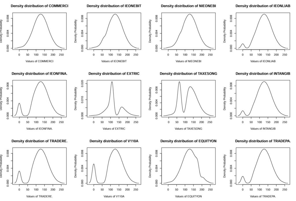
Histograms for ratios: DEBTEQU,CURRENT,QUICKRA,SALESONV,SALESMIN,ROAMINUS,EBITDAIE,EQUILIABL,DEBTEQUTR,ROETR (Density_wcs9train.ratiosG-25-34.pdf)
Proceeding with LDA (Linear Discriminant Analysis
The printed output is:# Preparing datatable for LDA analysis wcs9trainGL <- cbind(wcs9train$BADGOOD, wcs9train.ratiosG) names(wcs9trainGL)[1] <- “BADGOOD” # Running LDA on all variables with equal “a priori” probabilities for groups “Bad” and “Good” library(MASS) # Removing rows with NA w <- na.omit(wcs9trainGL) z <- lda(BADGOOD ~ ., data=w, prior = c(1,1)/2, CV = TRUE) tab <- table(w$BADGOOD, z$class) tab
| Group code | “Bad” | “Good” |
|---|---|---|
| “Bad” | 20 | 31 |
| “Bad” | 331 | 885 |
NOTE : It is fairly good result ! in terms of BAD but rather “conservative” in terms of GOOD