
Compliance Testing - Fairness Assessment using R
- Compliance Testing - Fairness Assessment using R
- Preprocessing - Semantic tagging using the LSEG-PermID (Open Calais) service
- Step1 - Load data and libraries
- Step 2 – Perform Principal Component Analysis (PCA) and evaluate clustering potential
- Step 3 - Perform K-means on a factor scores sub-space at evaluate performance with a minimum number of clusters
- Step 4 - Display retained clusters statistics
- Step5 - Evaluate fairness of Basing Hall-BIC selection process
We follow: K-Means Clustering in R: Algorithm and Practical Examples (https://www.datanovia.com/en/lessons/k-means-clustering-in-r-algorith-and-practical-examples/)
We need to extract the 2 factor sores vectors for components 2-3 following: get_pca: Extract the results for individuals/variables in Principal Component Analysis – R software and data mining (http://www.sthda.com/english/wiki/get-pca-extract-the-results-for-individuals-variables-in-principal-component-analysis-r-software-and-data-mining)
occ.pca.ind <- get_pca_ind(occ.pca)
occ.pca.ind <- occ.pca.ind$coord
occ.pca.23 <- occ.pca.ind[,c(2,3)]
df <- scale(occ.pca.23)
We follow: fviz_nbclust: Dertermining and Visualizing the Optimal Number of Clusters (https://www.rdocumentation.org/packages/factoextra/versions/1.0.7/topics/fviz_nbclust)
The best pratice is to compute a “clustering quality index” which is the sum of the inertia of clusters as a function of the number of clusters
A cluster “inertia” is its variance around its center (i.d., average cluster vector).
Starting from the variance of the whole cloud (one cluster), the sum of the inertia of clusters tends to decrease and stabilize as the number of clusters increases. The “elbow rule” advises to retain the number of clusters where the curve has reached its stable level.
fviz_nbclust(df, kmeans, method = “wss”) +
geom_vline(xintercept = 3, linetype = 2)
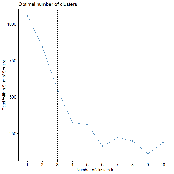
-> INTERPRETATION -> The generated plot shows a significant bend at 4-5 clusters
-> The analysis continues using 5 clusters